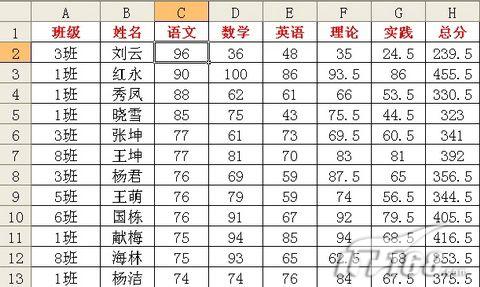
schools often organize examinations after the end of each test is a rule on performance analysis and comparison. Each class is the highest score for each subject the data to compare one, then in Excel 2003, how to quickly get needed data? The following methods you try.

we worksheet shown in Figure 1 as an example. Classes in the "raw scores" A worksheet columns, language, and the score of all subjects listed in the C-H column. We will not sort the original list, screening operation on the basis of each class the highest score of all subjects.

Figure 1 Excel worksheet in the original

one, start the PivotTable

click menu command "Data ¡ú PivotTable and PivotChart" start "PivotTable and PivotChart Wizard." A total of three steps, first select the "Microsoft Office Excel data list or database" single-option and the "pivot table" one option; the second step in the "selected areas" input box, enter the cell where the data area range "$ A $ 1: $ H $ 109"; the last step select the "New Sheet" option in order to produce a single PivotTable into a new worksheet. Click "Finish" button to open a new worksheet, and get the view shown in Figure 2 results.

Figure 2 Excel starts the PivotTable $ show_page $

Second, statistical score the highest score

in the "PivotTable Field List" dialog box, select the "class" project, drag it to the view, "the line Fields Here", release the mouse, you can get the class list. The "language" project drag "items Here Please", then "Mathematics" also Here. Received at this time is the sum of the two disciplines each class achievements, and the two disciplines are arranged in parallel position up and down, very convenient. We can use the mouse to drag the PivotTable in the "Data" button to the right of the "summary" Department, as shown in Figure 3 can be placed side by side so that the two disciplines. All subjects and then drag the data of other areas, we hope that you can quickly form on the.

Figure 3 Excel to set performance summary

But now each class of statistics is the sum result of all disciplines is not the best. However, it is very easy to change. Shown in Figure 4, first click on B5: B13 range of cells in a cell, and then click on "Pivot Table" toolbar button second from the left "field settings", then open the "Pivot style name Section "dialog box, select" summary manner "to" maximum "to determine the language after each class can seek to score the highest marks. Other subjects follow suit, on the line.

If you do not see "PivotTable" toolbar, just click the menu command "View ¡ú Toolbars ¡ú Pivot Table" can be seen.